Linear Regression
Linear Regression shows the Linear Relationship between dependent features(Y-axis) and independent features(X-axis).
There are 2 types of Linear Regression:
1. Simple Linear Regression -
It has only one independent variable.
Hypothesis Function for Simple Linear Regression :

where:
- Y is the dependent variable
- X is the independent variable
- β0 is the intercept ( the value where the regression line crosses the y-axis)
- β1 is the slope/weight
.png)
2. Multiple Linear Regression -
Hypothesis Function for Simple Linear Regression :
y= a0 + a1x1 + a2x2 + a3x3 + ..
Let's understand this by example, we all know that if the size of the house is bigger, then the price also increases. But along with this, there are many other factors that matters such as area and condition of the house. Here is a figure for that

if the equation is like y= 2+ 3x1+5x2+2x3
then, we can say that feature x2 is more important than others.
then, we can say that feature x2 is more important than others.
Remember, the more the weight, the more the feature is important.
- Positive Linear Regression

- Negative Linear Regression
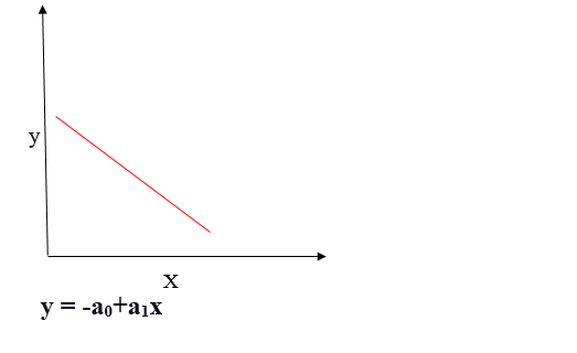
- Aim of Linear Regression
Cost function for Linear Regression


Why are we performing square?
Suppose the actual data points are [3,2,4] and predicted results are [5,3,2].
so, the error will be [2,1,-2] , now, without squaring , if we take mean , 2 and (-2) will be cancelled out, and we will get the less error compared to actual error. so, we have to square the distance.
Model is performing good if the MSE is closer to zero.
In order to get best fit line, we have to keep changing the values of a1 & a2(theta1 and theta2).
- Gradient Descent
Gradient descent is a method of updating a0 and a1 to minimize the cost function (MSE). We perform a random selection of coefficient values and then iteratively update the values to reach the minimum cost function.
.png)
We should always look for Global Minima as at that value of theta, we will have a line which is very near to actual data.
- How to find Global Minima?
Using, Convergence Algorithm.
Let’s differentiate the cost function(J) with respect to theta1.
![\begin {aligned} {J}'_{\theta_1} &=\frac{\partial J(\theta_1,\theta_2)}{\partial \theta_1} \\ &= \frac{\partial}{\partial \theta_1} \left[\frac{1}{n} \left(\sum_{i=1}^{n}(\hat{y}_i-y_i)^2 \right )\right] \\ &= \frac{1}{n}\left[\sum_{i=1}^{n}2(\hat{y}_i-y_i) \left(\frac{\partial}{\partial \theta_1}(\hat{y}_i-y_i) \right ) \right] \\ &= \frac{1}{n}\left[\sum_{i=1}^{n}2(\hat{y}_i-y_i) \left(\frac{\partial}{\partial \theta_1}( \theta_1 + \theta_2x_i-y_i) \right ) \right] \\ &= \frac{1}{n}\left[\sum_{i=1}^{n}2(\hat{y}_i-y_i) \left(1+0-0 \right ) \right] \\ &= \frac{1}{n}\left[\sum_{i=1}^{n}(\hat{y}_i-y_i) \left(2 \right ) \right] \\ &= \frac{2}{n}\sum_{i=1}^{n}(\hat{y}_i-y_i) \end {aligned}](https://quicklatex.com/cache3/bf/ql_333278a99944456db14b39cd9fe7b7bf_l3.svg "Rendered by QuickLaTeX.com")
Let’s differentiate the cost function(J) with respect to theta2.
![\begin {aligned} {J}'_{\theta_2} &=\frac{\partial J(\theta_1,\theta_2)}{\partial \theta_2} \\ &= \frac{\partial}{\partial \theta_2} \left[\frac{1}{n} \left(\sum_{i=1}^{n}(\hat{y}_i-y_i)^2 \right )\right] \\ &= \frac{1}{n}\left[\sum_{i=1}^{n}2(\hat{y}_i-y_i) \left(\frac{\partial}{\partial \theta_2}(\hat{y}_i-y_i) \right ) \right] \\ &= \frac{1}{n}\left[\sum_{i=1}^{n}2(\hat{y}_i-y_i) \left(\frac{\partial}{\partial \theta_2}( \theta_1 + \theta_2x_i-y_i) \right ) \right] \\ &= \frac{1}{n}\left[\sum_{i=1}^{n}2(\hat{y}_i-y_i) \left(0+x_i-0 \right ) \right] \\ &= \frac{1}{n}\left[\sum_{i=1}^{n}(\hat{y}_i-y_i) \left(2x_i \right ) \right] \\ &= \frac{2}{n}\sum_{i=1}^{n}(\hat{y}_i-y_i)\cdot x_i \end {aligned}](https://quicklatex.com/cache3/b8/ql_2000092923a5e57a510faeb99a907eb8_l3.svg "Rendered by QuickLaTeX.com")

Here, alpha is a learning rate and the value inside bracket is called as slope.
Now, there is a possibility that we can get -ve or +ve slope.
- If we have +ve slope,
.png)
a1 = a1 - alpha(+ve)
so, here a1 will get reduced and move towards global minima.
- If we have -ve Slope,
.png)
a1 = a1 - alpha(-ve)
so, here a1 will get increased and move towards global minima.
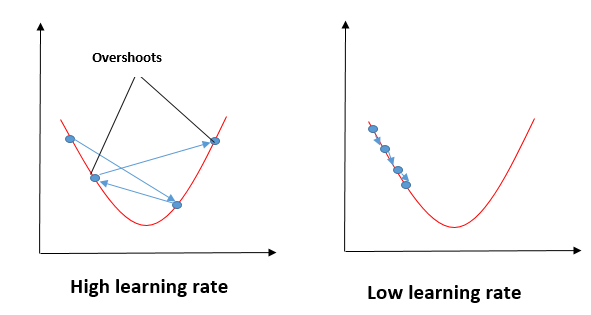
- Learning Rate -
If the learning rate is too slow, it will take a lot of time to reach at global minima & if it is so high than it might skip the global minima.
- In Deep Learning, we can face the problem of local minima, but in Gradient Descent you will always find Global minima because the graph of Gradient Descent is 'U' shaped.
- R-Squared -
Let's take one example, consider p=no. of features
i. p=2 -> Bedroom, Price -> R-Squared=81%
ii. p=3 -> Bedroom, Price, location -> R-Squared=90%
iii. p=4 -> Bedroom, Price, location, Gender -> R-Squared=93%
R-Squared increases as the no. of features gets increased. But, if you look at the last example, notice that Gender is not relevant to predict the price of a flat. So, if we use R-Squared only, we might come to wrong conclusions.
That's where Adjusted R-Squared comes in picture.
- Adjusted R-Squared -
Where:
- is the number of samples,
- is the number of features.
- Adjusted R-squared values range from 0 to 1, with higher values indicating a better fit of the model.
- Assumptions of Linear Regression
- 1. Linearity:
- The relationship between the independent and dependent variables is linear.
- 2. Independence:
- The residuals (the differences between the actual and predicted values) are independent of each other. This means that the error in predicting Y for one observation must not related to the error in predicting Y for another observation.
- 3. Homoscedasticity:
- The variance of the residuals is constant across all levels of the independent variables. This indicates that the amount of the independent variable(s) has no impact on the variance of the errors.
- 4. Normality:
- The residuals are normally distributed. This means that the residuals should follow a bell-shaped curve.


Comments
Post a Comment