Logistic Regression
.png)
Logistic Regression is used when our dependent variable is dichotomous or binary. It just means a variable that has only 2 outputs, for example, The student will pass this exam or not.
It is also used in multiclass classification. For example, Will you attend the seminar? [Yes, Maybe, No]
Types of Logistic Regression:
1) Binary logistic regression
It is used to predict the probability of a binary outcome, such as yes or no, true or false, or 0 or 1
2) Multinomial logistic regression
It is used to predict the probability of one or more possible outcomes, such as the type of product a customer will buy [cheap, costly, affordable, popular]
3) Ordinal logistic regression
It is used to predict the probability of an outcome that falls into a predetermined order, such as the level of customer satisfaction, the severity of a disease, or the stage of cancer.
Why to use Logistic Regression instead of Linear Regression?
Let's understand this by an example:
Suppose, if study hours > 1.8 => pass, else => fail
Now, if you create a model for this condition, using linear regression, then for the good inputs it will work, but if there are outliers, in that case, our model will not predict correct output.


The graph of linear regression is a straight line, where as for logistic regression, the graph is 'S - shaped'.
Sigmoid or Logistic Function:-

equation of the best fit line in linear regression is:
Let’s say instead of y, we are taking probabilities (P). But there is an issue here, the value of (P) will exceed 1 or go below 0 and we know that range of Probability is (0-1). To overcome this issue we take “odds” of P.
The odds of an event happening is defined as the probability of the event divided by the probability of the event not happening:
log of odds which has a range from (-∞,+∞) and Odds are always in range (0,+∞ ) so, how do we get the range of probability P which is (0,1)?


Assumptions of Logistic Regression:
Binary outcome:
It is used when dependent variable is dichotomous (e.g., 0 or 1, yes or no).Independence of observations: The outcome of one observation should not be influenced by the outcome of another observation.
Linearity of independent variables and log odds: The relationship between the independent variables and the log odds of the dependent variable should be linear.
No multicollinearity: Multicollinearity occurs when two or more independent variables are highly correlated, which can make it difficult to determine the effect of each variable on the outcome.
Large sample size: To ensure that the model is not overfitting the data.
No outliers: Outliers can affect the estimates of the coefficients in logistic regression, so it's important to check and address outliers in the dataset.
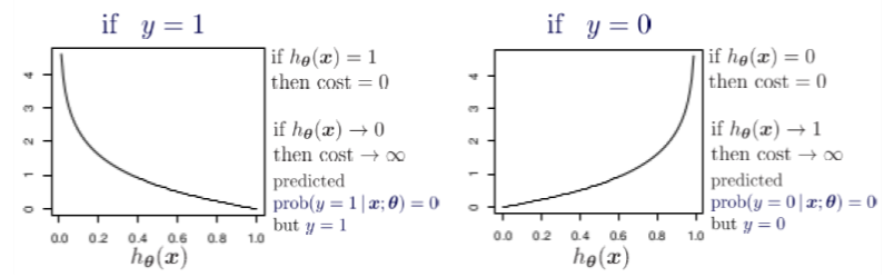
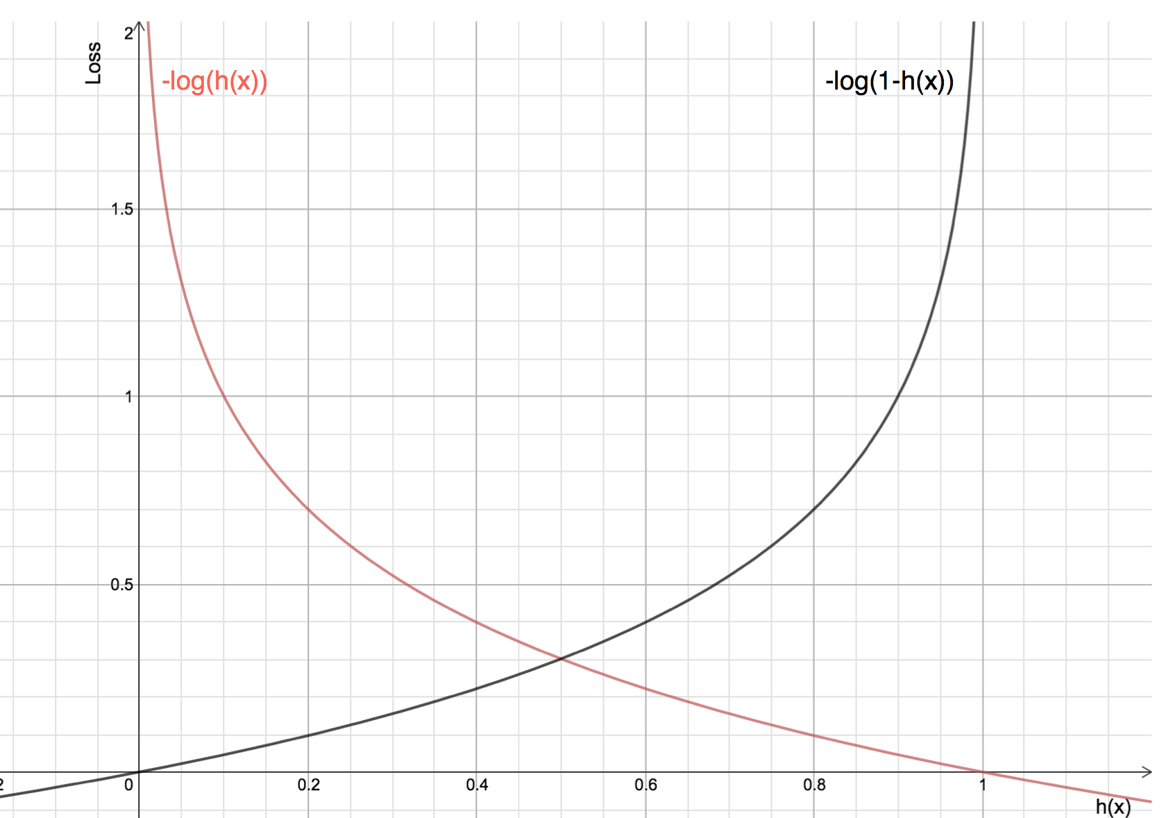
Cost Function in Logistic Regression


Let’s see what will be the graph of cost function when y=1 and y=0


Comments
Post a Comment